machine learning for finance - part 2

In this series of posts I’m trying some of the ideas in the book Advances in Financial Machine Learning, by Marcos López de Prado. Here I tackle an idea from chapter 5: fractional differencing.

the problem

Stock prices are nonstationary - their means and variances change systematically over time. Take for instance the price of BOVA11 (an ETF that tracks Brazil’s main stock market index, Ibovespa):

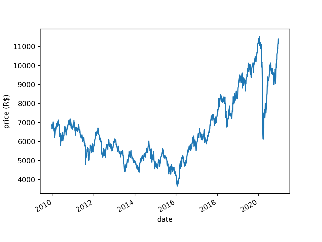
There is a downward trend in BOVA11 prices between 2010 and 2016, then an upward trend between 2016 and 2020. Unsurprisingly, the Augmented Dickey-Fuller (ADF) test fails to reject the null hypothesis of nonstationarity (p=0.83).

(When I say that the mean and variance change “systematically” in a nonstationary series I don’t mean that in a stationary series the mean and variance are exactly the same at all times. With any stochastic process, stationary or not, the mean and variance will vary - randomly - over time. What I mean is that in a nonstationary series the parameters of the underlying probability distribution - the distribution that is generating the data - change over time. In other words, in a nonstationary series the mean and variance change over time not just randomly, but also systematically. Before the math police come after me, let me clarify that this a very informal definition. In reality there are different types of stationarity - weak, strong, ergodic - and things are more complicated than just “the mean and variance change over time”. Check William Greene’s Econometric Analysis, chapter 20, for a mathematical treatment of the subject.)

Why does stationarity matter? It matters because it can trip your models. If BOVA11 prices are not stationary then whatever your model learns from 2010 BOVA11 prices is not generalizable to, say, 2020. If you just feed the entire 2010-2020 time series into your model its predictions may suffer.

Most people handle nonstationarity by taking the first-order differences of the series. Say the price series is \(\begin{vmatrix}y_{t0}=100 & y_{t1}=105 & y_{t2}=97\end{vmatrix}\). The first-order differences are \(\begin{vmatrix}y_{t1}-y_{t0}=105-100=5 & y_{t2}-y_{t1}=97-105=-8\end{vmatrix}\).

You can take differences of higher order too. Here the second-order differences would be \(\begin{vmatrix}-8-5=-13\end{vmatrix}\). But taking first-order differences often achieves stationarity, so that’s what most people do with price data.

If you take the first-order differences of the BOVA11 series you get this:

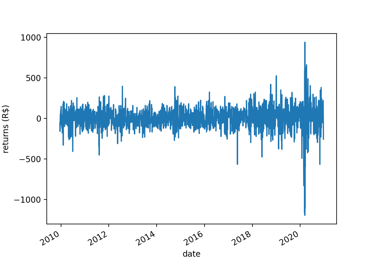
This looks a lot more “stable” than the first plot. Here the ADF test rejects the null hypothesis of nonstationarity (p<0.001).

The problem is, by taking first-order differences you are throwing the baby out with the bathwater. Market data has a low signal-to-noise ratio. The little signal there is is encoded in the “memory” of the time series - the accumulation of shocks it has received over the years. When you take first-order differences you wipe out that memory. To give an idea of the magnitude of the problem, the correlation between BOVA11 prices and BOVA11 returns is a mere 0.06. As de Prado puts it (p. 76):

The dilemma is that returns are stationary, however memory-less, and prices have memory, however they are non-stationary.

what to do?

de Prado’s answer is fractional differencing. Taking first-order differences is “integer differencing”: you are taking an integer \(d\) (in this case 1) and you are differencing the time series \(d\) times. But as de Prado shows, you don’t have to choose between \(d=0\) (prices) and \(d=1\) (returns). \(d\) can be any rational number between 0 and 1. And the lower \(d\) is the less memory you wipe out when you difference the time series.

With an integer \(d\) you just subtract yesterday’s price from today’s price and that’s it, you have your first-order difference. But with a non-integer \(d\) you can’t do that. You need a differencing mechanism that works for non-integer \(d\) values as well. I show one such mechanism in the next section.

some matrix algebra

First you need to abandon scalar algebra and switch to matrix algebra. Let’s not worry about fractional differencing just yet. Let’s just answer this: what sorts of matrices and matrix operations would take a vector \(\begin{vmatrix}x_{t0} & x_{t1} & x_{t2} ... x_{tN}\end{vmatrix}\) and return the \(d\)th-order differences of those \(N\) elements?

Say that your price vector is \(X=\begin{vmatrix}5 & 7 & 11\end{vmatrix}\). The first matrix you need here is an identity matrix of order \(N\). If it’s been a while since your linear algebra classes, an identity matrix is a square matrix (a matrix with the same number of rows and columns) that has 1s in its main diagonal and 0s everywhere else. Here your vector has 3 elements, so your identity matrix needs to be of order 3. Here it is:

You also need a second matrix, \(B\). Like \(I\), \(B\) is also a square matrix of order \(N\) with 1s in one diagonal and 0s elsewhere. But unlike in \(I\), in \(B\) the first row is all 0s; the 1s are in the subdiagonal, not in the main diagonal:

As it turns out, you can use \(I\) and \(B\) to difference \(X\). The first step is to compute \(I - B\):

Now you raise \(I - B\) to the \(d\)th power. Let’s say you want to find the second-order differences. In that case \(d=2\). Well, if \(d=2\) you could simply multiply \(I - B\) by \(I - B\), like this:

But that is not a very general solution - it only works for an integer \(d\). So instead of multiplying \(I - B\) by itself like that you are going to resort to a little trick you learned back in grade 10:

where \(k = 0, 1, ... n\)

That is called the binomial theorem. If you apply it to \((I - B)^d\) you get

where \(k = 0, 1, ... d\)

(In case you’re wondering, \(I^{d-k}\) disappeared because an identity matrix raised to any power is itself, and because an identity matrix multiplied by any other matrix is that other matrix. Hence \(I^{d-k} (-B)^k = I(-B)^k = (-B)^k\))

(Before someone calls the math police: the binomial theorem only extends to matrices when the two matrices are commutative, i.e., when \(XY=YX\). In fractional differencing that is always going to be the case, as \(I\) is an identity matrix and that means \(XI=IX\) for any matrix \(X\). But outside the context of fractional differencing you need to take a look at this paper.)

The binomial expands like this:

If \(d=2\) that means

…which is the same result we had obtained by simply multiplying \(I - B\) by itself.

Now you multiply \((I - B)^d\) by your original vector, \(X\). Here this means:

Finally, you discard the first \(d\) elements of that product (I’ll get to that in a moment) and what’s left are your second-order differences. That means your vector of second-order differences is \(\begin{vmatrix}2\end{vmatrix}\). Voilà!

That’s a lot of matrix algebra to do what any fourth-grader can do in a matter of seconds. Very well then, let’s use fourth-grade math to check the results. If your vector is \(\begin{vmatrix}5 & 7 & 11\end{vmatrix}\) then the first-order differences are \(\begin{vmatrix}7-5 & 11-7\end{vmatrix}\) \(=\begin{vmatrix}2 & 4\end{vmatrix}\) and the second-order differences are \(\begin{vmatrix}4-2\end{vmatrix}=\begin{vmatrix}2\end{vmatrix}\). Check!

With matrix algebra you get \(\begin{vmatrix}5 & -3 & 2\end{vmatrix}\) instead of \(\begin{vmatrix}2\end{vmatrix}\) because the matrix operations carry the initial \(5\) all the way through, which means that at some point the difference \(2 - 5\) is computed even though it makes no real-world sense. That’s why you need to discard the initial \(d\) elements of the final product.

If you want to reproduce all that in Python here is the code:

import numpy as np

def get_I_and_B(X):
    n = X.shape[0]
    I = np.identity(n)
    row0 = np.zeros((1, n))
    B = np.vstack((row0, I[:n-1]))
    return I, B

def difference_method1(X, d):
    I, B = get_I_and_B(X)
    return np.matmul(np.linalg.matrix_power(I - B, d), X)

def difference_method2(X, d):
    I, B = get_I_and_B(X)
    w0 = I
    w1 = -d * B
    w2 = np.linalg.matrix_power(B, 2)
    W = w0 + w1 + w2
    return np.matmul(W, X)

X = [5, 7, 11]
X = np.array(X)
d = 2

diffs = difference_method1(X, d)
print(diffs)
diffs = difference_method2(X, d)
print(diffs)

The point of using all that matrix algebra and the binomial theorem is that \((I - B)^d X\) works both for an integer \(d\) and for a non-integer \(d\). Which means you can now compute, say, the 0.42th-order differences of a time series. The only thing that changes with a non-integer \(d\) is that the series you saw above becomes infinite:

Finding \(\sum_{k=0}^{\infty} \binom{d}{k} (-B)^k\) can be computationally expensive, so people usually find an approximation instead. There are different ways to go about that and de Prado discusses some alternatives in his book. But at the end of the day you’re still computing \((I - B)^d\), same as you do for integer \(d\) values. Multiply the result by \(X\) and you have your fractional differences. Just remember to discard the first element of the resulting vector (you can’t discard, say, 0.37 elements; you have to round it up to 1).

I thank mathematician Tzanko Matev, whose tutorial helped me understand fractional differencing. If I made any mistakes here they are all mine.

quick note

de Prado arrives at \(\sum_{k=0}^{\infty} \binom{d}{k} (-B)^k\) through a different route that requires fewer steps. Here it is, from page 77:

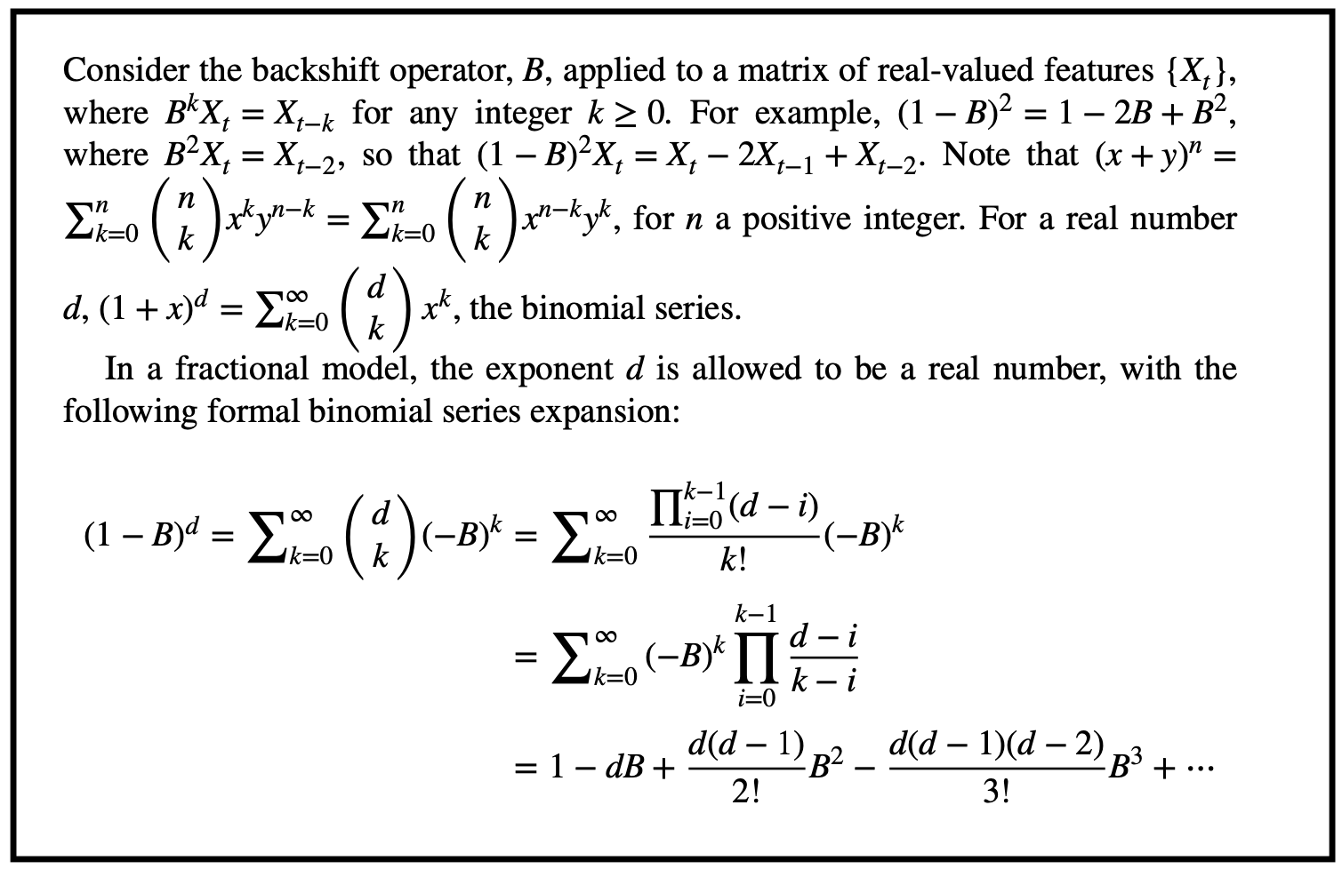
The way he does it is certainly more concise. But I found that by doing the matrix algebra in a more explicit way, and by including a few more intermediate steps, I understood the whole thing much better.

how to choose d

Alright, so a non-integer \(d<1\) will erase less memory than an integer \(d\geq1\), and now you know the math behind fractional differences. But how do you choose \(d\)? de Prado suggests that you try different values of \(d\), apply the ADF test on each set of results, and pick the lowest \(d\) that passes the test (p<0.05).

Time to work then. de Prado includes Python scripts for everything in his book, so you could simply use that. But here I want to try a more optimized and production-ready implementation. I couldn’t find anything like that for Python. But I found a nifty R package - fracdiff. It’s well documented and it uses an optimization trick that makes it run fast (the optimization is based on a 2014 paper - A Fast Fractional Difference Algorithm, by Andreas Jensen and Morten Nielsen -, with tweaks by Martin Maechler).

I do almost everything in Python these days and I didn’t want to deal with RStudio, dplyr, etc, just for this one thing. So I wrote almost the entire code in Python, and then inside my Python code I have this one string that is my R code, and I use a package called rpy2 to call R from inside Python.

Here is the full code. It reads the BOVA11 dollar bars that I created in my previous post (and saved here for your convenience), generates the plots and statistics I used in the beginning of this post, and finds the best \(d\).

import numpy as np
import pandas as pd
from rpy2 import robjects
from matplotlib import pyplot as plt
from statsmodels.tsa.stattools import adfuller

# load data
df = pd.read_csv('bars.csv')

# fix date field
df['date'] = pd.to_datetime(df['date'], format = '%Y-%m-%d')

# sort by date
df.index = df['date']
del df['date']
df = df.sort_index()

# plot
df['closing_price'].plot(ylabel = 'price (R$)', xlabel = 'date')
plt.show()
df['closing_price'].diff().dropna().plot(ylabel = 'returns (R$)', xlabel = 'date')
plt.show()

# check if series is stationary
def check_stati(y):
    y = np.array(y)
    p = adfuller(y)[1]
    return pvalue

# prices
check_stati(df['closing_price'].values)

# returns
check_stati(df['closing_price'].diff().dropna().values)

# check correlation
c = np.corrcoef(df['closing_price'].values[1:], df['closing_price'].diff().dropna().values)
print(c)

# stringify vector of prices
# (so we can put it inside R code)
vector = ', '.join([str(e) for e in list(df['closing_price'])])

# try several values of d
ds = []
d = 0
got_it = False
while d < 1:

    # differentiate!
    rcode = '''
    library('fracdiff')
    diffseries(c({vector}), {d})
    '''.format(vector = vector, d = d)
    output = robjects.r(rcode)

    # check correlation between prices and differences
    c = np.corrcoef(output[1:], df['closing_price'].values[1:])[1][0]

    # check if prices are stationary
    p = check_stati(output)

    # appendd and c (to plot later)
    ds.append((d, c))

    if (not got_it) and (p < 0.05):
        print(' ')
        print('d:', d)
        print('c:', c)
        got_it = True

    d += 0.01

Running this code you find that the lowest \(d\) that passes the ADF test is 0.29. Much lower than the \(d=1\) most people use when differencing a price series.

With \(d=0.29\) the correlation between the price series and the differenced series is 0.87. In contrast, the correlation between the price series and the return series (\(d=1\)) was 0.06. In other words, with \(d=0.29\) you are preserving a lot more memory - and therefore signal.

As an addendum, the script also plots how the correlation between prices and \(d\)-order differences decreases as we increase \(d\):

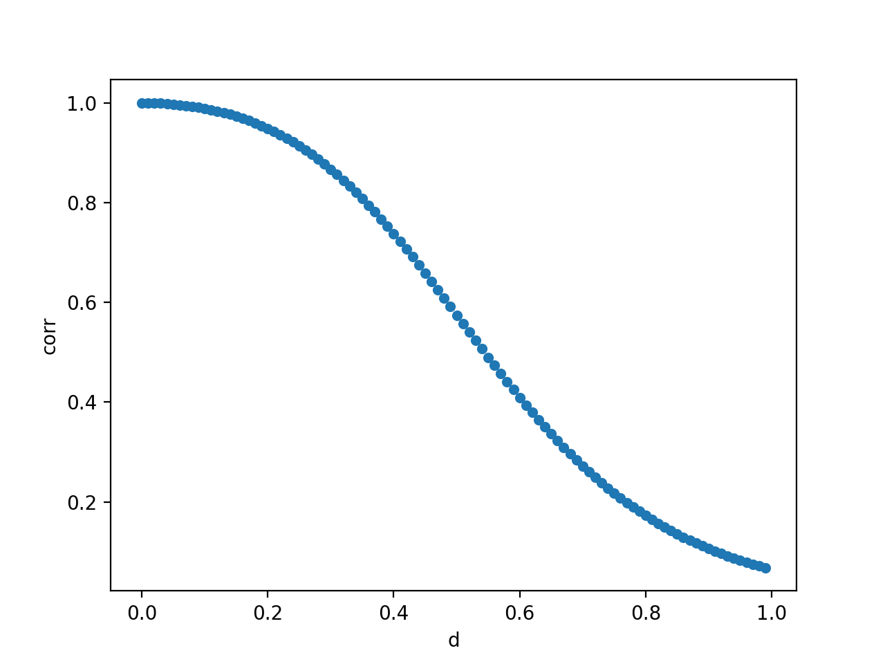
Clearly the lower \(d\) is the more memory you preserve.

This is it! See you on the next post.