Getting historical intraday financial data can be a pain, especially for non-US markets. If you have deep pockets you can simply buy the data you need, but for retail investors the cost is prohibitive. If you want historical transaction-level data for the Brazilian stock market, for instance, TickData will sell it to you for about US$ 65000. Hard pass. What to do?
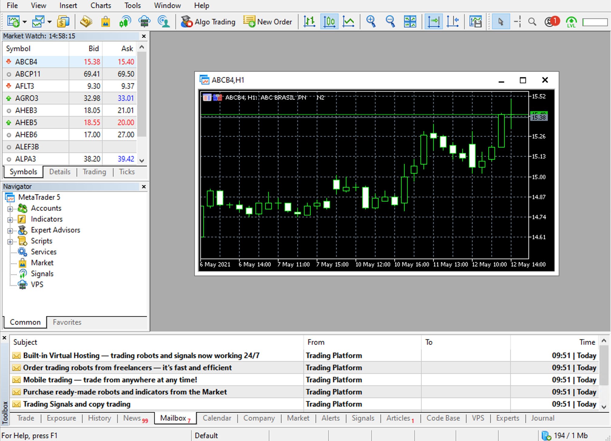
I recently learned about an app called MetaTrader. MetaTrader gives you real-time stock price charts. It is popular with people who do technical analysis - people who buy and sell equities based on certain chart patterns (like a “head and shoulder formation”, for instance). I’ve never bothered with technical analysis and I guess that’s why MetaTrader had escaped my radar until now.
The important thing is: many brokers pay MetaTrader so that their clients can access it, and MetaTrader has historical intraday data for whatever market(s) each broker operates in.
I checked and it turns out that my broker in Brazil has one such deal with MetaTrader. I got a username and password, downloaded the app, and started exploring.
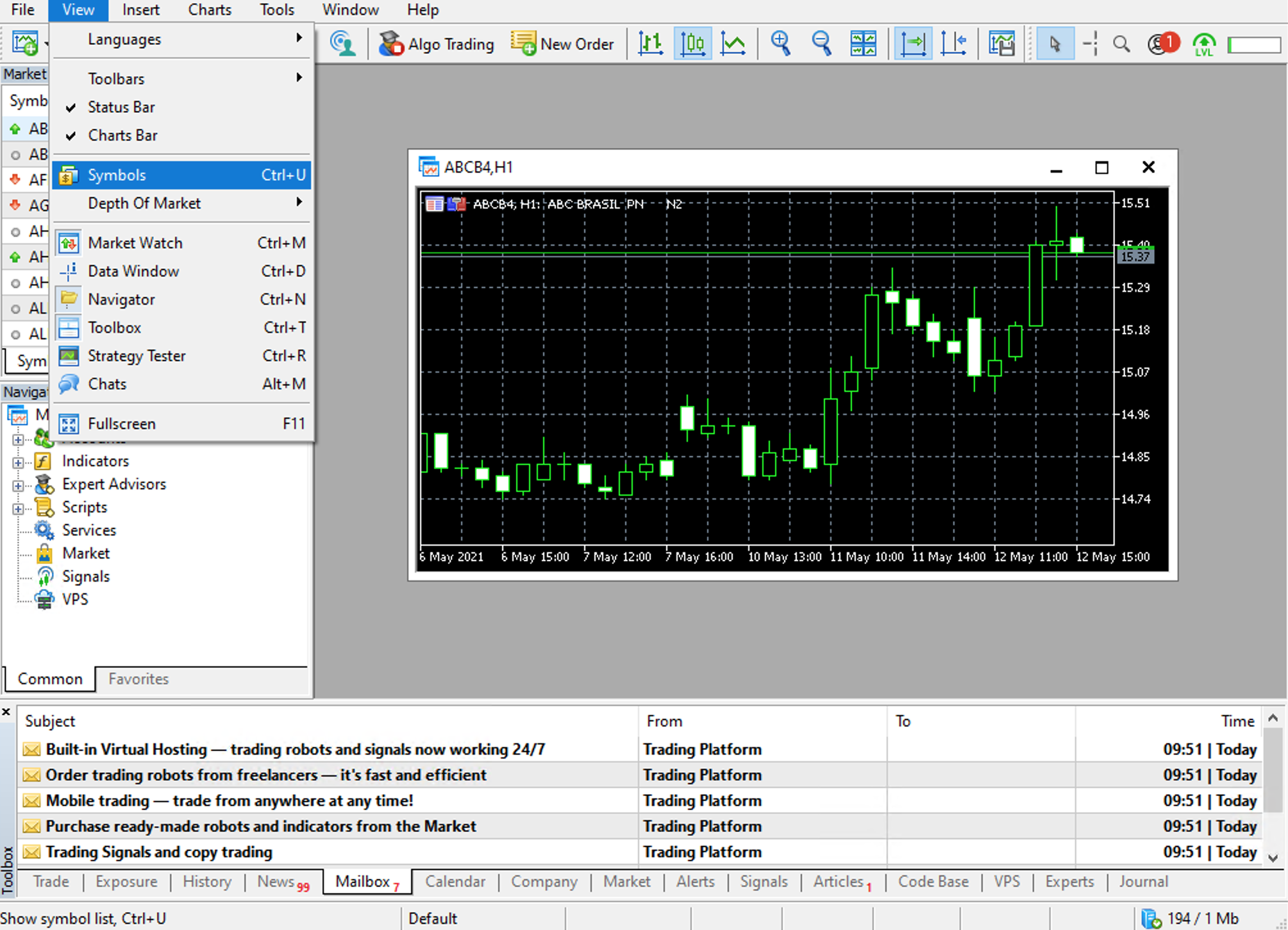
If you’re only interested in a couple of equities you can export the data manually. Go to the View menu and click Symbols.
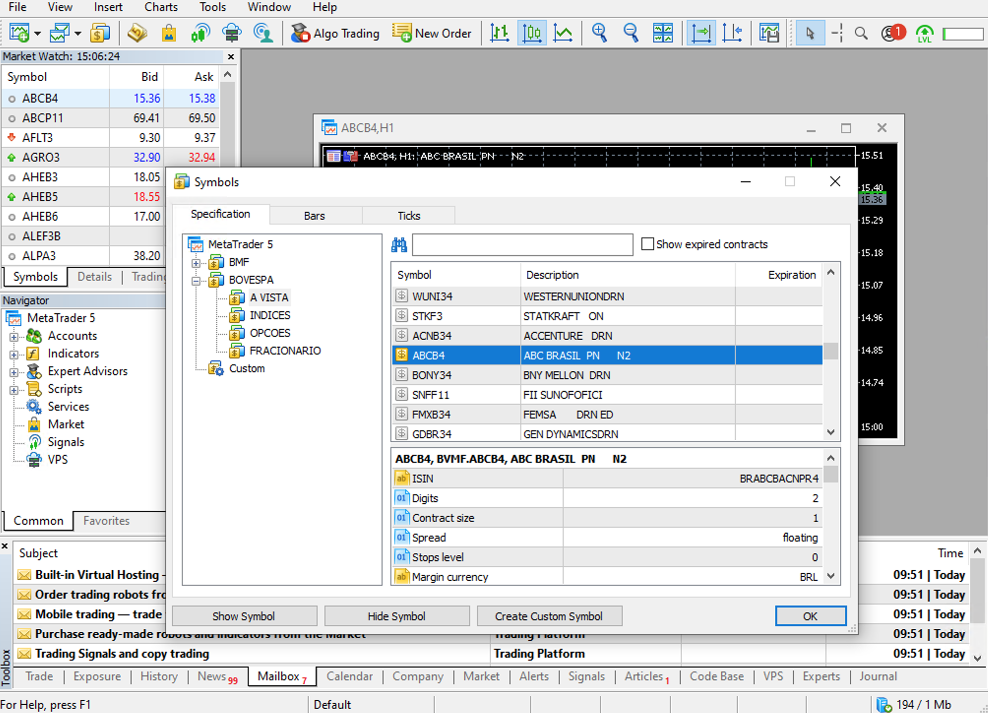
A new window will open:
The “BMF” and “Bovespa” you see in that window are the names of two exchanges in Brazil (they’ve been merged into a single exchange called B3 but I guess MetaTrader is keeping the old names for now). You will see different names, depending on where your broker operates.
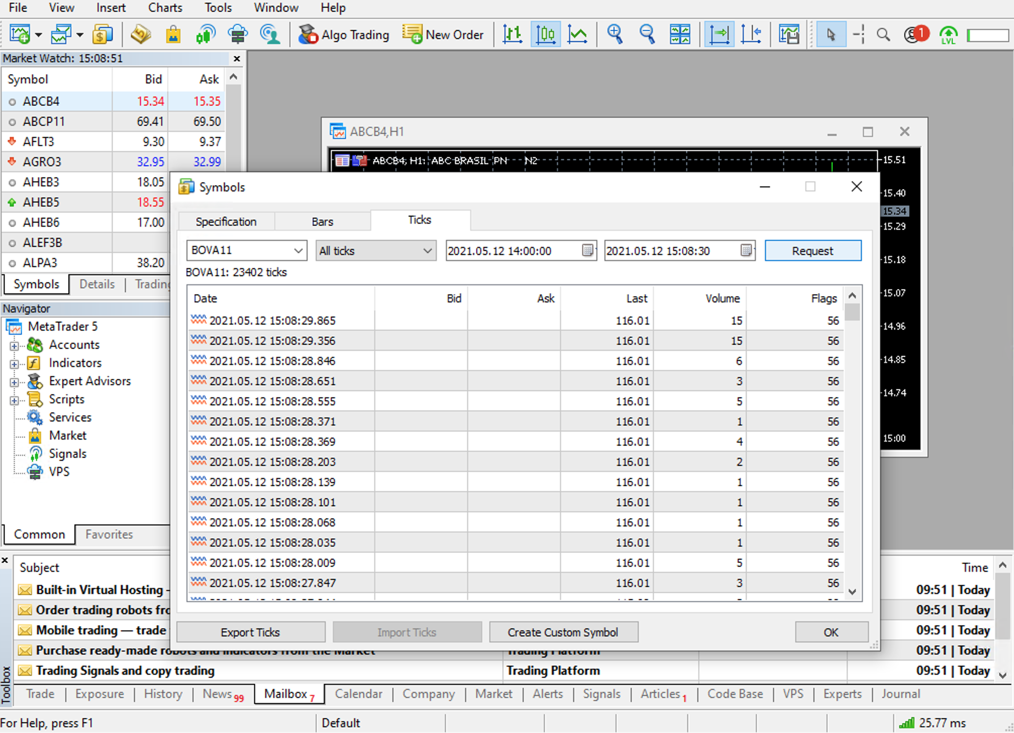
Say you’re interested in tick data. Just click on the Ticks tab, enter the ticker for the equity you want, and click Request. Here I am requesting tick data for BOVA11, an ETF that tracks Brazil’s main stock market index:
The Export Ticks button lets you save the data in a CSV format.
If you want time bars then go to the Bars tab instead.
The data you get depends on what your broker provides MetaTrader. I explored a bit and it looks like lower frequency data requests yield longer time series. When I request 1-minute BOVA11 bars I only get a year or so of data, but when I request 5- or 10-minute BOVA11 bars I get a few more years. That’s a far cry from the 13 years of data TickData sells, but for us DIY wannabe quants that’s enough to play around a bit. And, well, it costs zero dollars. (With TickData you’d need to pay US$ 6750 to access a single year of tick data from Brazil).
That’s all there is to it - if you are only interested in a couple of equities. But what if you want data for hundreds of equities? Or for all equities? Fortunately, MetaTrader has a nice Python API that you can access after pip installing the MetaTrader5 package.
Unfortunately, the MetaTrader5 package only works on Windows. If you want to use it on a macOS or Linux machine you’ll need Wine. I have access to a Windows machine so that wasn’t a problem for me.
Here is a minimal working example of how the Python API works. This snippet requests tick data (trade ticks only - no bid/ask ticks) for BOVA11 between 2021-01-01 and 2021-01-07 and then saves the results in a CSV file. Before you run this script you need to launch the MetaTrader app and log into it using the credentials your broker gave you.
importpandasaspdimportMetaTrader5asmt5fromdatetimeimportdatetime,timedelta# connect to MetaTrader 5
ifnotmt5.initialize():print('initialize() failed')mt5.shutdown()# request tick data
ticks=mt5.copy_ticks_range('BOVA11',datetime(2021,1,1),datetime(2021,1,7),mt5.COPY_TICKS_TRADE)ticks=pd.DataFrame(ticks)ticks.to_csv('BOVA11_ticks.csv',index=False)# shut down connection to MetaTrader 5
mt5.shutdown()
If you want data for more equities just loop through the corresponding tickers. If that’s a lot of tickers there is a method symbols_get() that will return all tickers. For instance, the tickers for Brazilian ordinary stocks always have four letters followed by the number 3 - PETR3, HYPE3, etc. If you want only ordinary stocks you can use symbols_get() and then filter out any string that doesn’t have five characters or doesn’t end in 3.
One issue I’ve come across is that sometimes the API returns no data even though a manual search (using the GUI) shows that there is data. That doesn’t happen often but when it does it’s always with highly liquid equities, so I’m guessing if there is too much data to return you get nothing instead. So you may want to loop through shorter intervals - months instead of quarters, or weeks instead of months, or days instead of weeks, depending on how much data you’re requesting.
Another thing to keep in mind is that MetaTrader generates temp files for your requests and they are big as heck. It got to the point where my hard drive ran out of space. I had to use Python’s os to delete those temp files on-the-fly. They are saved to AppData/Roaming/MetaQuotes/Terminal/HASH/bases/BrokerID/ by default. If you want them to be saved elsewhere you have to move the MetaTrader installation folder to the new location and then execute it using cmd, with AlternateLocation/terminal64.exe /portable The temp files will be stored in AlternateLocation/Bases/BrokerID/
Here is a more complete example:
importosimporttimeimportcalendarimportpandasaspdimportMetaTrader5asmt5fromdatetimeimportdatetime,timedelta# connect to MetaTrader 5
ifnotmt5.initialize():print('initialize() failed')mt5.shutdown()# get connection status and parameters
print(mt5.terminal_info())# get MetaTrader 5 version
print(mt5.version())# path to CSVs
path_to_csvs='C:/Users/YourUserName/Desktop/ticks/'# path to temp data (so we can delete it)
path_to_tmp='C:/Users/YourUserName/AppData/Roaming/MetaQuotes/Terminal/HASH/bases/BrokerID/'# get all B3 tickers
symbols=mt5.symbols_get()# keep only tickers for ordinary stocks
tickers=[]forsymbolinsymbols:ticker=symbol.nameifnotticker[:4].isalpha():continueif(len(ticker)==5)and(ticker[-1]=='3'):tickers.append(ticker)# month-years to scrape
months={2019:(10,11,12),2020:range(1,13),2021:(1,2,3)}# loop through tickers
start=time.time()fori,tickerinenumerate(tickers):# loop through month-years
foryearinmonths.keys():formonthinmonths[year]:print(' ')print(i,'of',len(tickers),ticker,year,month)# set date range
t0=datetime(year,month,1)last_day=calendar.monthrange(year,month)[1]t1=datetime(year,month,last_day)# request tick data
ticks=mt5.copy_ticks_range(ticker,t0,t1,mt5.COPY_TICKS_TRADE)ticks=pd.DataFrame(ticks)# log if results are empty
ifticks.shape[0]==0:withopen('log.txt',mode='a')asf:l=ticker+','+str(year)+','+str(month)+'\n'f.write(l)print('empty DataFrame:',l)continue# persist
print(ticks.shape[0])ticks['time']=pd.to_datetime(ticks['time'],unit='s')ticks.columns=['ticktime','bid','ask','last','volume','time_msc','flags','volume_real']ticks.to_csv(path_to_csvs+ticker,index=False)# don't over-request
time.sleep(2.5)# delete tmp files
forfnameinos.listdir(path_to_tmp+ticker+'/'):try:os.remove(path_to_tmp+ticker+'/'+fname)except:pass# how long did it take?
elapsed=time.time()-startprint('it took',round(elapsed/60),'minutes')# shut down connection to MetaTrader 5
mt5.shutdown()
Finally, a word about the “flags” column (you can see it in the BOVA11 screenshot above). That column encodes a lot of information. For instance, it encodes whether the tick refers to a buy-initiated trade or to a sell-initiated trade. But it’s not as simple as “56 means buy-initiated” or anything like that. It took me some doing to learn how to interpret the flags. Turns out they are bit masks. To extract the information encoded in each flag you need to do a bunch of bitwise operations. For instance, to tell whether a given tick represents a buy- or sell-initiated trade you need to pass the flag through a function like this:
defbuy_or_sell(flag):'''
see https://www.mql5.com/en/forum/75268
for explanation on MetaTrader flags
'''if(flag&32)and(flag&64):return'both'elifflag&32:return'buy'elifflag&64:return'sell'
MetaTrader uses 32 to encode “buy-initiated” and 64 to encode “sell-initiated”. Say the flag for a given tick is 56. The bitwise operation 56 AND 64 returns 0. That means the tick does not refer to a sell-initiated trade. But the bitwise operation 56 AND 32 returns 32. That means the tick refers to a buy-initiated trade. (In some rare cases the tick refers to a trade that was simultaneously initiated by buyer and seller.) The flag 212, on the other hand, returns opposite results: 212 AND 32 returns 0 and 212 AND 64 returns 64 - in other words, a tick with the flag 212 refers to a sell-initiated trade.
Here is information on everything else that each flag encodes.
This is it. Let me know if there are other sources of intraday data I should check out. What are the cool kids using?
I just finished Jack Schwager’s Unknown Market Wizards. It’s a collection of interviews with retail traders. The interviewees follow different approaches - fundamental, technical, quant, social media mining - but they share similar attitudes and Schwager does a good job hypothesizing how these attitudes might relate to trading outcomes. On top of that, Schwager is a superb interviewer and he shows the world of retail traders in a way that’s neither the aggregate statistics of academic papers nor the get-rich-quick Youtube ads selling day trading courses. I’ve always thought of traders as people who somehow missed Burton Malkiel’s A Random Walk Down Wall Street. Schwager showed me a much more interesting picture. Here are some highlights:
skill vs luck
The eleven traders in the book all have spectacular performances. We’re talking annualized returns of 20%-300%, sometimes for several years. But the book doesn’t give us enough data to know whether those performances are the result of skill or mere luck. If you ride a big bull market it’s possible to have stellar returns with random bets. Bitcoin has yielded an annualized return of 558% since May 2015. That doesn’t make early Bitcoin adopters market wizards (though some of them certainly are).
“The magnitude by which the traders in this book outperformed market benchmarks over long periods (typically, decade-plus) cannot simply be explained away as ‘luck.’”, Schwager writes (p. 348). To give only two examples, Daljit Dhaliwal never had a negative year and he was profitable in 95% of quarters, and Pavel Krejcí had positive returns in 93% of all quarters. But to tell luck from skill we would need to know who was trading what when and what each monthly return was, then follow an approach like Fama & French’s where they compare actual returns with simulated returns. Schwager doesn’t give us a data appendix, so we can’t do that. (The data is not Schwager’s to publicize but he could have run the numbers himself and showed us the results.)
It’s tempting to guess which of the eleven traders are skilled (as opposed to merely lucky) based on the narrative each of them offers. Several of them emphasize the importance of updating your beliefs based on new information (so that you can limit your losses if the market turns against you, for instance), but without overcorrecting. Some also emphasize the importance of sizing your bets according to how confident you are. These attitudes are typical of Philip Tetlock’s superforecasters.
But they are just narratives. Each trader (except for the one quant guy) is describing his mental model of himself. That mental model is probably a better trader than the actual human behind it. And at times the narratives sound wishy-washy: “I am using my feelings as an input to trading.” (p. 110), “The human emotions that we feel can be used as a signal source.” (p. 193), that sort of thing. (Though for the most part the narratives are pretty Tetlockian.)
In short, it is possible that Schwager selected eleven very lucky people and then spent hours listening to after-the-fact rationalizations. But even if that’s the case (which I don’t know) the book is still immensely enjoyable if you are curious about retail trading.
people who are always wrong can make (you) money
My favorite strategy is one of Jason Shapiro’s:
I watch Fast Money religiously at 5 p.m. EST every day. I can’t tell you how much money I’ve made off of that show. […] There is one guy on the program named Brian Kelly, who I have now watched for years. He is wrong by such a larger percentage than random that it is hard to believe. I will never have a position on if he is recommending it. (p. 69)
I don’t know if that really works or if Shapiro is just rationalizing but I love the idea and now I want to find Fast Money transcripts and backtest it.
shrinking anomalies
Several of the interviewees believe that anomalies are disappearing.
Peter Brandt, talking about how things have changed for chartists since the 1980s:
Large long-term patterns no longer work. Trendlines no longer work. Channels no longer work. Symmetrical triangles no longer work. (p. 37)
Richard Bargh:
there are also far fewer opportunities now than back in 2013 and 2014. Back then, many things were still relatively new, like quantitative easing and forward guidance. There was more uncertainty about what the central banks were going to do and how they were going to do it. Whereas now, the markets have central banks so nailed down that there is not as much opportunity to make money on central banks as there once was. The markets now are good at pricing in events before they happen. I make money by pricing in a surprise, and with fewer surprises, there are fewer opportunities. (p. 100)
Amrit Sall:
increased market automation and high-frequency-trading algorithms have made execution harder and eroded my edge on some very short time frame strategies. (p. 142)
Daljit Dhaliwal:
It is no longer possible to trade for the initial move off the headline because the algos will make the trade before I can. (p. 157)
It makes sense. Data is cheaper, processing power is cheaper, machine learning courses are free; it would be odd if anomalies didn’t disappear.
patience
Another common theme is the importance of waiting for the right trade.
Richard Bargh says you should have a side project:
One thing about event-driven trading is that if there isn’t an event to trade, there is nothing to do, and it is really boring. You can feel like you’re wasting your life. […] I have found that I trade much better when I have a side project. If I have nothing else to do but trade events, and there are no events to trade, my mind runs wild. I need to focus my attention on something; otherwise, I will focus on the wrong things. (p. 104)
Bargh again:
Trading to earn a consistent amount steadily may be an admirable goal, but it is not a realistic one. Market opportunities are sporadic. […] If you try to force consistent profitability, you will be prone to take suboptimal trades, which will often end up reducing your overall profitability. (p. 177)
Amrit Sall:
There will be periods in the markets where opportunities dry up, and there will be nothing to do. In those nothing periods, if you are looking for something to do, that is when you can create real damage to your account. (p. 129)
Daljit Dhaliwal:
you don’t have to take every potential trade. You can wait for a trade where everything lines up in your favor. (p. 154)
Chris Camillo articulated it best:
Looking back, I think a big part of my success when I went back to trading was my ability to look past the noise and be patient. I wasn’t in the industry. It wasn’t my job, and I wasn’t under any pressure to trade. I could go six months without a trade, and I didn’t have to answer to anybody. (p. 239)
(The other day I was listening to a podcast interview with a quant fund manager and he emphasized that “we work a lot, we don’t just create a bot and then go to the beach”. It’s odd that people choose to invest in a quant fund but then expect constant human activity - as long as the fund is making you money what do you care that the staff is at the beach? But apparently investors want busy managers.)
What Camillo says ties in with Marsten Parker’s advice:
Don’t quit your day job. (p. 287)
If you have a stable source of income it’ll probably be easier to avoid overtrading.
TickerTags
One of my favorite interviews in the book is the one with Chris Camillo. He mines social media looking for information that might help him anticipate stock price movements. Like when there was an outbreak of E. Coli in Chipotle stores:
Chipotle had become famous for having long lines at lunchtime. Chipotle was such a trendy brand that it was common for people to tweet about having lunch there. They would also frequently tweet about how they were waiting in line at Chipotle. I was able to gauge real-time foot traffic by monitoring word combinations, such as “Chipotle” plus “lunch,” and “Chipotle” plus “line,” in online conversations. Almost overnight, the mentions of these word combinations dropped by about 50%.
I imagine NLP folks at quant shops reading about Camillo and his Chipotle trade. There they are, fine-tuning BERT and whatnot, and then Camillo with his hard-coded bigrams makes a killing.
Camillo made a business out of that: he created TickerTags, a company that tracks word combinations on social media. As Camillo says, tracking conversations is a way to “go even earlier than trasactional data” (like credit card information).
TickerTags doesn’t seem to have been successful with hedge funds though:
Hedge fund managers want something repeatable and systematic. They wanted to know how often this approach would generate tradable information with high conviction. I couldn’t give them a hard answer. (p. 253)
That is a recurrent theme throughout the book. The trader “knows” that the strategy works but somehow can’t put a number on it. Peter Brandt says if the market closes in a new high or in a new low on a Friday then it is likely to keep moving in that direction on Monday and early Tuesday. But when asked if he ever checked that pattern he replies “I have never statistically analyzed it.” Hhmm.
the one quant guy
Marsten Parker is the only quant in the group. He touches on an interesting point:
I’ve always struggled with how to distinguish between a routine drawdown and a system that has stopped working. (p. 278)
Last month I finished reading Marcos López de Prado’s Advances in Financial Machine Learning. de Prado talks about how the death of a strategy can actually be a good thing:
For instance, a mean-reverting pattern may give way to a momentum pattern. As this transition takes place, most market participants are caught off guard, and they will make costly mistakes. This sort of errors is the basis for many profitable strategies, because the actors on the losing side will typically become aware of their mistake once it is too late. Before they accept their losses, they will act irrationally, try to hold the position, and hope for a comeback. Sometimes they will even increase a losing position, in desperation. Eventually they will be forced to stop loss or stop out. Structural breaks offer some of the best risk/rewards. (p. 249)
de Prado suggests a number of tests to identify structural breaks - for instance, testing if the cumulative forecasting errors look random. I wonder if that’s the sort of thing Parker is doing. He doesn’t get into technical details though, other than to mention that he’s learned about overfitting the hard way, that he uses parameter stability as an indicator of robustness, that your errors will be more serially correlated in real life than in your backtest, and that it’s best to have several simple strategies than one over-optimized strategy. (Also: “The more strategies you run, the easier it is emotionally to turn one off.”, p. 286.)
I love this:
if I knew everything I do now, I might never have tried trading in the first place. (p. 286)
I imagine all the state-of-the-art models that RenTec or AQR must be training, the hordes of Mensa Ph.D.s they recruit, the deep pockets they have to buy credit card data or Twitter’s Firehose, I think of Quantopian’s failure, and it sounds impossible to me that any sort of artisanal, DIY quant approach could succeed. But maybe Parker isn’t just lucky. His interview updated my priors a bit.
loving your trade
The appeal of trading is that it is something you can do on your own - no employees, no bosses, no clients, no students, no reviewers, no drama, no politics, no culture wars.
Jason Shapiro:
I had six people working for me, and I hated it. I didn’t like managing people and being responsible for their success. (p. 72)
Pavel Krejcí:
I wanted to find something where the success or failure would depend only on me, not my colleagues, my boss, or anybody else. If I make money, that’s great; if I lose money, it’s my mistake. (p. 320)
That’s happinness almost by definition.
Alright, any more quotes and I’ll probably get a lawsuit so I’m stopping here. Go buy the book.
In this series of posts I’m trying some of the ideas in the book Advances in Financial Machine Learning, by Marcos López de Prado. Here I tackle an idea from chapter 5: fractional differencing.
the problem
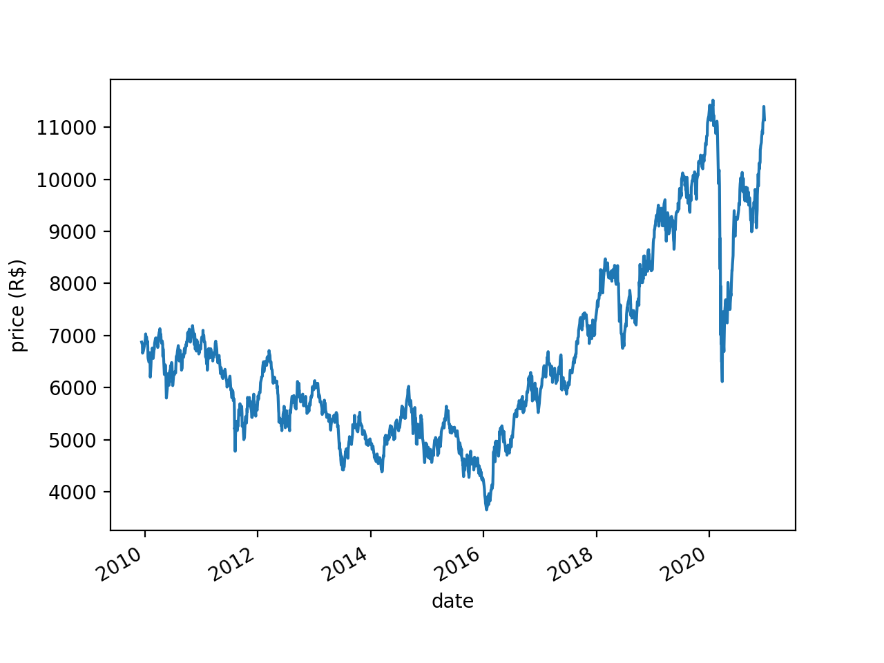
Stock prices are nonstationary - their means and variances change systematically over time. Take for instance the price of BOVA11 (an ETF that tracks Brazil’s main stock market index, Ibovespa):
There is a downward trend in BOVA11 prices between 2010 and 2016, then an upward trend between 2016 and 2020. Unsurprisingly, the Augmented Dickey-Fuller (ADF) test fails to reject the null hypothesis of nonstationarity (p=0.83).
(When I say that the mean and variance change “systematically” in a nonstationary series I don’t mean that in a stationary series the mean and variance are exactly the same at all times. With any stochastic process, stationary or not, the mean and variance will vary - randomly - over time. What I mean is that in a nonstationary series the parameters of the underlying probability distribution - the distribution that is generating the data - change over time. In other words, in a nonstationary series the mean and variance change over time not just randomly, but also systematically. Before the math police come after me, let me clarify that this a very informal definition. In reality there are different types of stationarity - weak, strong, ergodic - and things are more complicated than just “the mean and variance change over time”. Check William Greene’s Econometric Analysis, chapter 20, for a mathematical treatment of the subject.)
Why does stationarity matter? It matters because it can trip your models. If BOVA11 prices are not stationary then whatever your model learns from 2010 BOVA11 prices is not generalizable to, say, 2020. If you just feed the entire 2010-2020 time series into your model its predictions may suffer.
Most people handle nonstationarity by taking the first-order differences of the series. Say the price series is \(\begin{vmatrix}y_{t0}=100 & y_{t1}=105 & y_{t2}=97\end{vmatrix}\). The first-order differences are \(\begin{vmatrix}y_{t1}-y_{t0}=105-100=5 & y_{t2}-y_{t1}=97-105=-8\end{vmatrix}\).
You can take differences of higher order too. Here the second-order differences would be \(\begin{vmatrix}-8-5=-13\end{vmatrix}\). But taking first-order differences often achieves stationarity, so that’s what most people do with price data.
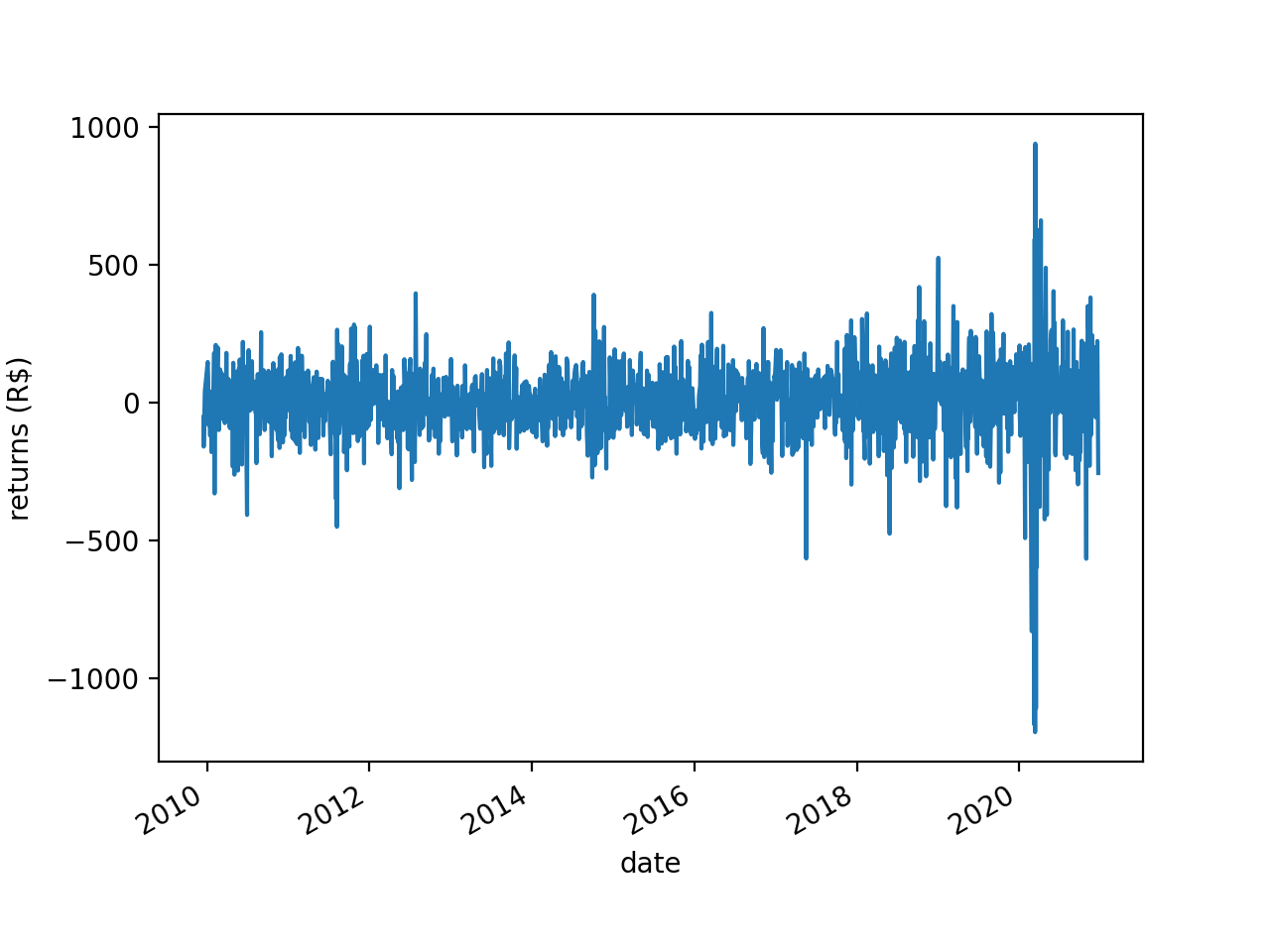
If you take the first-order differences of the BOVA11 series you get this:
This looks a lot more “stable” than the first plot. Here the ADF test rejects the null hypothesis of nonstationarity (p<0.001).
The problem is, by taking first-order differences you are throwing the baby out with the bathwater. Market data has a low signal-to-noise ratio. The little signal there is is encoded in the “memory” of the time series - the accumulation of shocks it has received over the years. When you take first-order differences you wipe out that memory. To give an idea of the magnitude of the problem, the correlation between BOVA11 prices and BOVA11 returns is a mere 0.06. As de Prado puts it (p. 76):
The dilemma is that returns are stationary, however memory-less, and prices have memory, however they are non-stationary.
what to do?
de Prado’s answer is fractional differencing. Taking first-order differences is “integer differencing”: you are taking an integer \(d\) (in this case 1) and you are differencing the time series \(d\) times. But as de Prado shows, you don’t have to choose between \(d=0\) (prices) and \(d=1\) (returns). \(d\) can be any rational number between 0 and 1. And the lower \(d\) is the less memory you wipe out when you difference the time series.
With an integer \(d\) you just subtract yesterday’s price from today’s price and that’s it, you have your first-order difference. But with a non-integer \(d\) you can’t do that. You need a differencing mechanism that works for non-integer \(d\) values as well. I show one such mechanism in the next section.
some matrix algebra
First you need to abandon scalar algebra and switch to matrix algebra. Let’s not worry about fractional differencing just yet. Let’s just answer this: what sorts of matrices and matrix operations would take a vector \(\begin{vmatrix}x_{t0} & x_{t1} & x_{t2} ... x_{tN}\end{vmatrix}\) and return the \(d\)th-order differences of those \(N\) elements?
Say that your price vector is \(X=\begin{vmatrix}5 & 7 & 11\end{vmatrix}\). The first matrix you need here is an identity matrix of order \(N\). If it’s been a while since your linear algebra classes, an identity matrix is a square matrix (a matrix with the same number of rows and columns) that has 1s in its main diagonal and 0s everywhere else. Here your vector has 3 elements, so your identity matrix needs to be of order 3. Here it is:
You also need a second matrix, \(B\). Like \(I\), \(B\) is also a square matrix of order \(N\) with 1s in one diagonal and 0s elsewhere. But unlike in \(I\), in \(B\) the first row is all 0s; the 1s are in the subdiagonal, not in the main diagonal:
Now you raise \(I - B\) to the \(d\)th power. Let’s say you want to find the second-order differences. In that case \(d=2\). Well, if \(d=2\) you could simply multiply \(I - B\) by \(I - B\), like this:
But that is not a very general solution - it only works for an integer \(d\). So instead of multiplying \(I - B\) by itself like that you are going to resort to a little trick you learned back in grade 10:
(In case you’re wondering, \(I^{d-k}\) disappeared because an identity matrix raised to any power is itself, and because an identity matrix multiplied by any other matrix is that other matrix. Hence \(I^{d-k} (-B)^k = I(-B)^k = (-B)^k\))
(Before someone calls the math police: the binomial theorem only extends to matrices when the two matrices are commutative, i.e., when \(XY=YX\). In fractional differencing that is always going to be the case, as \(I\) is an identity matrix and that means \(XI=IX\) for any matrix \(X\). But outside the context of fractional differencing you need to take a look at this paper.)
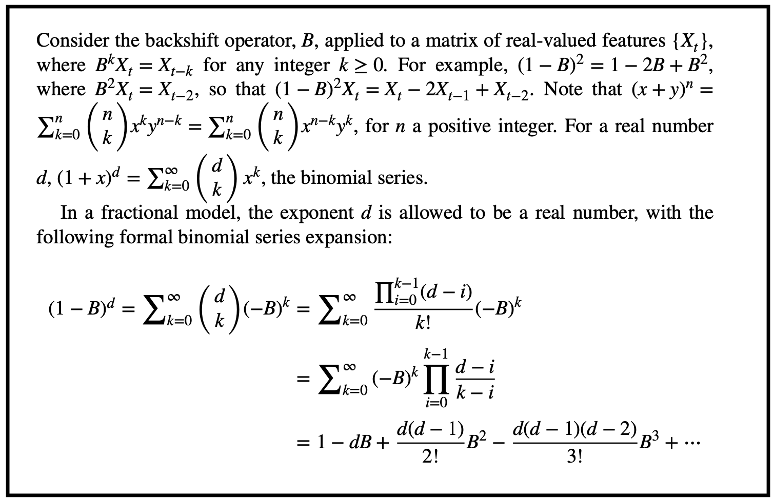
The binomial expands like this:
\[\sum_{k=0}^{d} \binom{d}{k} (-B)^k = I - dB + \dfrac{d(d-1)}{2!}B^{2} - \dfrac{d(d-1)(d-2)}{3!} B^3 + ...\]
Finally, you discard the first \(d\) elements of that product (I’ll get to that in a moment) and what’s left are your second-order differences. That means your vector of second-order differences is \(\begin{vmatrix}2\end{vmatrix}\). Voilà!
That’s a lot of matrix algebra to do what any fourth-grader can do in a matter of seconds. Very well then, let’s use fourth-grade math to check the results. If your vector is \(\begin{vmatrix}5 & 7 & 11\end{vmatrix}\) then the first-order differences are \(\begin{vmatrix}7-5 & 11-7\end{vmatrix}\) \(=\begin{vmatrix}2 & 4\end{vmatrix}\) and the second-order differences are \(\begin{vmatrix}4-2\end{vmatrix}=\begin{vmatrix}2\end{vmatrix}\). Check!
With matrix algebra you get \(\begin{vmatrix}5 & -3 & 2\end{vmatrix}\) instead of \(\begin{vmatrix}2\end{vmatrix}\) because the matrix operations carry the initial \(5\) all the way through, which means that at some point the difference \(2 - 5\) is computed even though it makes no real-world sense. That’s why you need to discard the initial \(d\) elements of the final product.
If you want to reproduce all that in Python here is the code:
The point of using all that matrix algebra and the binomial theorem is that \((I - B)^d X\) works both for an integer \(d\) and for a non-integer \(d\). Which means you can now compute, say, the 0.42th-order differences of a time series. The only thing that changes with a non-integer \(d\) is that the series you saw above becomes infinite:
\[\sum_{k=0}^{\infty} \binom{d}{k} (-B)^k\]
Finding \(\sum_{k=0}^{\infty} \binom{d}{k} (-B)^k\) can be computationally expensive, so people usually find an approximation instead. There are different ways to go about that and de Prado discusses some alternatives in his book. But at the end of the day you’re still computing \((I - B)^d\), same as you do for integer \(d\) values. Multiply the result by \(X\) and you have your fractional differences. Just remember to discard the first element of the resulting vector (you can’t discard, say, 0.37 elements; you have to round it up to 1).
I thank mathematician Tzanko Matev, whose tutorial helped me understand fractional differencing. If I made any mistakes here they are all mine.
quick note
de Prado arrives at \(\sum_{k=0}^{\infty} \binom{d}{k} (-B)^k\) through a different route that requires fewer steps. Here it is, from page 77:
The way he does it is certainly more concise. But I found that by doing the matrix algebra in a more explicit way, and by including a few more intermediate steps, I understood the whole thing much better.
how to choose d
Alright, so a non-integer \(d<1\) will erase less memory than an integer \(d\geq1\), and now you know the math behind fractional differences. But how do you choose \(d\)? de Prado suggests that you try different values of \(d\), apply the ADF test on each set of results, and pick the lowest \(d\) that passes the test (p<0.05).
Time to work then. de Prado includes Python scripts for everything in his book, so you could simply use that. But here I want to try a more optimized and production-ready implementation. I couldn’t find anything like that for Python. But I found a nifty R package - fracdiff. It’s well documented and it uses an optimization trick that makes it run fast (the optimization is based on a 2014 paper - A Fast Fractional Difference Algorithm, by Andreas Jensen and Morten Nielsen -, with tweaks by Martin Maechler).
I do almost everything in Python these days and I didn’t want to deal with RStudio, dplyr, etc, just for this one thing. So I wrote almost the entire code in Python, and then inside my Python code I have this one string that is my R code, and I use a package called rpy2 to call R from inside Python.
Here is the full code. It reads the BOVA11 dollar bars that I created in my previous post (and saved here for your convenience), generates the plots and statistics I used in the beginning of this post, and finds the best \(d\).
importnumpyasnpimportpandasaspdfromrpy2importrobjectsfrommatplotlibimportpyplotaspltfromstatsmodels.tsa.stattoolsimportadfuller# load data
df=pd.read_csv('bars.csv')# fix date field
df['date']=pd.to_datetime(df['date'],format='%Y-%m-%d')# sort by date
df.index=df['date']deldf['date']df=df.sort_index()# plot
df['closing_price'].plot(ylabel='price (R$)',xlabel='date')plt.show()df['closing_price'].diff().dropna().plot(ylabel='returns (R$)',xlabel='date')plt.show()# check if series is stationary
defcheck_stati(y):y=np.array(y)p=adfuller(y)[1]returnpvalue# prices
check_stati(df['closing_price'].values)# returns
check_stati(df['closing_price'].diff().dropna().values)# check correlation
c=np.corrcoef(df['closing_price'].values[1:],df['closing_price'].diff().dropna().values)print(c)# stringify vector of prices
# (so we can put it inside R code)
vector=', '.join([str(e)foreinlist(df['closing_price'])])# try several values of d
ds=[]d=0got_it=Falsewhiled<1:# differentiate!
rcode='''
library('fracdiff')
diffseries(c({vector}), {d})
'''.format(vector=vector,d=d)output=robjects.r(rcode)# check correlation between prices and differences
c=np.corrcoef(output[1:],df['closing_price'].values[1:])[1][0]# check if prices are stationary
p=check_stati(output)# appendd and c (to plot later)
ds.append((d,c))if(notgot_it)and(p<0.05):print(' ')print('d:',d)print('c:',c)got_it=Trued+=0.01
Running this code you find that the lowest \(d\) that passes the ADF test is 0.29. Much lower than the \(d=1\) most people use when differencing a price series.
With \(d=0.29\) the correlation between the price series and the differenced series is 0.87. In contrast, the correlation between the price series and the return series (\(d=1\)) was 0.06. In other words, with \(d=0.29\) you are preserving a lot more memory - and therefore signal.
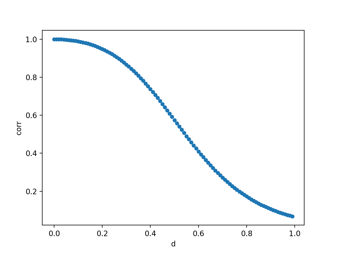
As an addendum, the script also plots how the correlation between prices and \(d\)-order differences decreases as we increase \(d\):
Clearly the lower \(d\) is the more memory you preserve.
I just finished a book called Advances in Financial Machine Learning, by Marcos López de Prado. It’s a dense book and I struggled with some of the chapters. Putting what I learned into practice (and explaining it in my own words) may help me grasp it better, so here it is. (Also, I thought it would be fun to try de Prado’s ideas on data from Brazil.) In this post I put into practice the idea of dollar bars (chapter 2). In the next post I will do fractional differencing (chapter 5). In later posts I want to do meta-labeling (chapter 3), backtesting with combinatorial cross-validation (chapter 12), and bet sizing (chapter 10).
basic idea
We normally think of time series data in terms of, well, time. In most time series each t is a day or a minute or a year or some other measure of time. But t can represent events instead. For instance, instead of t being 24 hours or 30 days or anything like that, it can be however long it takes for 100 people to walk by your house.
Let’s make that (admittedly silly) example more concrete. You wait by the window of your living room and start counting. It takes two hours for 100 people to walk by your house. You note that 28 of them were walking with dogs (let’s say that’s what you’re interested in). That’s it, you’ve collected your first sample: \(y_{t1}\) = 28/100 = 0.28. You start counting again. This time it takes only 45 minutes for another 100 people to walk by your house. 42 of them had dogs. That’s your second sample: \(y_{t2}\) = 42/100 = 0.42. And so on, until you have collected all the samples you want. The important thing to note here is that your t represents a variable amount of time. It’s two hours in the first sample but only 45 minutes in the second sample.
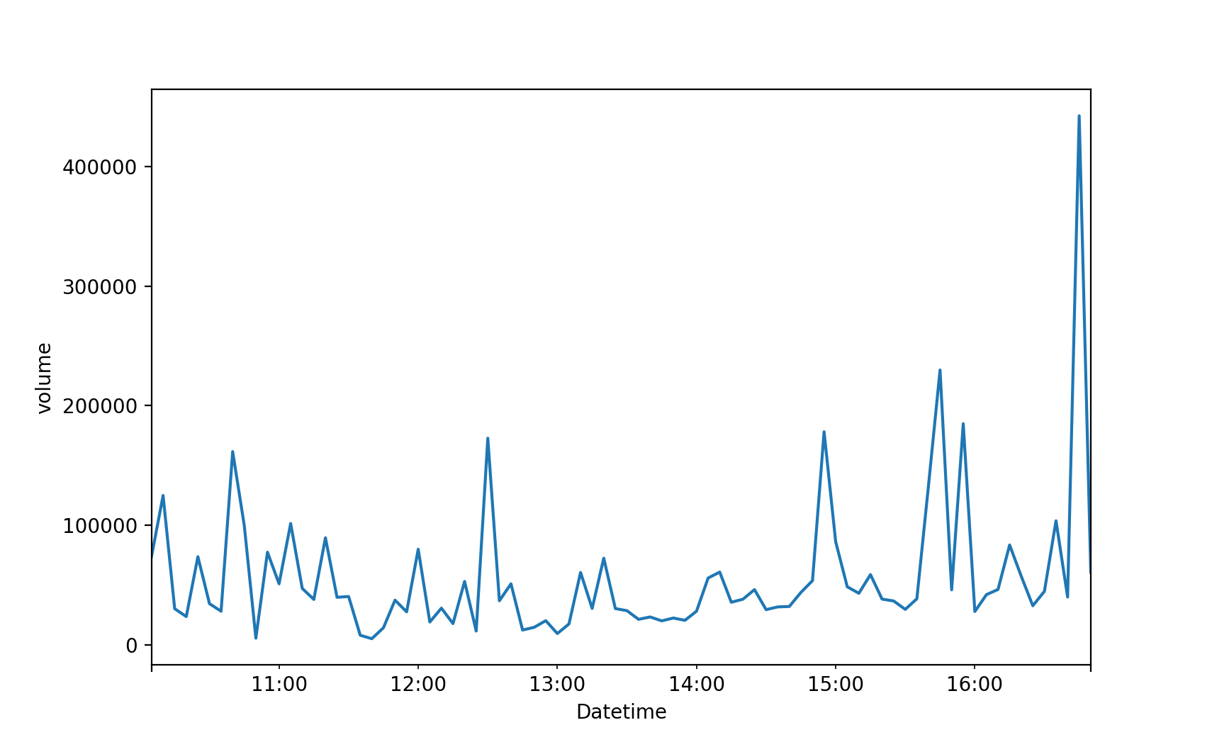
In finance most time series are built the conventional way, with t representing a fixed amount of time - like a day or an hour or a minute. de Prado shows that that creates a number of problems. First, it messes up sampling. The stock market is busier at certain times than others. Consider for example BOVA11, which is an ETF that tracks Brazil’s main stock market index (Ibovespa). This is how BOVA11 activity varied over time on April 12th, 2021:
As we see, some times of the day are busier than others. If t represents a fixed amount of time - 1 hour or 15 minutes or 5 minutes or what have you - you will be undersampling the busy hours and oversampling the less active hours.
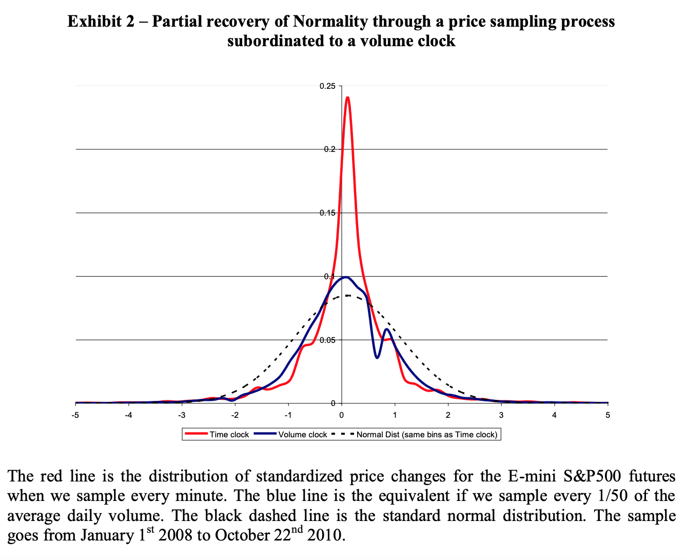
The second problem with using fixed time intervals, de Prado says, is that they make the data more serially correlated, more heteroskedastic, and less normally distributed. That may hurt the predictive performance of models like ARIMA. (I wonder whether those problems also hurt the performance of non-parametric models like random forest. The statistical properties of your coefficients can’t be affected when you have no coefficients. But I leave this discussion for another day.)
The solution de Prado offers is that we allow t to represent a variable amount of time - like in my silly example of counting passers-by. More specifically, de Prado suggests that we define t based on market activity. For instance, you can define t as “the time it takes for BOVA11 trades to reach R$ 1 million” (R$ is the symbol for reais, the currency of Brazil.) Say it’s 10am now and the stock market just opened. At 10:07 someone buys R$ 370k of BOVA11 shares. At 11:48 someone else buys another R$ 520k. That’s R$ 890k so far (370k + 520k = 890k). At 12:18, more R$ 250k. Bingo! The R$ 1 million threshold has been reached (370k + 520k + 250k = 1140k). You collect whatever data you are going to use in your model and you have your first sample. Say that you’re interested in the closing price and that it was R$ 100 at 12:18, when the R$ 1 million threshold was triggered. Then your first sample is \(y_{t1}\) = 100. You now wait for another R$ 1 million in BOVA11 trades to happen, so you can have your second sample. And so on.
In reality you don’t “wait” for anything, you look at past data and find the moments when the threshold was reached and then collect the information you want (closing price, volume, what have you).
You can collect more than one piece of information about each sample. Maybe you want closing price, average price, and volume. In that case your \(y_{t1}\) will be a vector of size 3 (as opposed to a scalar). In fact that is more common than collecting a single feature. And finance people often visualize each sample in the form of a “candlestick bar”, like this:
That’s why finance folks talk about “bars” instead of “samples” or “observations”. When the bars are based on fixed time intervals (5 minutes or 1 day or what have you) we call them “time bars”. When they are based on a variable amount of time that depends on a monetary threshold (like R$ 1 million or US$ 5 million) we call them “dollar bars”. (Apparently people call it “dollar bars” even if the actual currency is reais or euros or anything else.)
When you have collected all the samples (“bars”) you want you can use them in whatever machine learning model you choose. Suppose those samples are your y - the thing you want to predict. In that case you will normally want your X - your features - to be based on the same time intervals. In the example above our first sample corresponds to the interval between 10:00 and 12:18 of some day. Say you’re using tweets as one of your features. You will need to collect tweets posted between 10:00 and 12:18 of that same day. Suppose that it took two hours for another R$ 1 million in BOVA11 trades to happen. Then you will need to collect tweets posted between 12:18 and 14:18 of that day. And so on, until you have time-matching X data points for each y data point.
de Prado suggests other types of market-based bars, like tick bars (based on a certain number of trades) and volume bars (based on a certain number of shares traded). Here I’ll stick to dollar bars. Also, to keep things simple I will collect a single feature (closing price) from each sample.
how to make dollar bars
Ok, how do we create dollar bars with real-world data?
First snag: getting the data is hard. Brazil’s main stock exchange, B3, only publicizes daily data. That gives us, for each day and security, highly aggregated information like closing price and total volume. Ideally we would want intraday data - all that same information, but for each 1-minute interval or 5-minute interval. It’s not that I want to do high-frequency trading, it’s just that with intraday data I can train a wider range of models.
(Just to clarify: the goal here is to make dollar bars, not time bars. But I need time bars to build dollar bars.)
Yahoo Finance does give us intraday data (that’s how I got the data for the BOVA11 volume plot above), but only for the last 60 days. That means your models will give a lot of weight to whatever quirks the market experienced over the last 60 days.
You can subscribe to data providers like Economatica, which gives you intraday data going back many years. But that costs about US$ 5k a year. Hard pass. I don’t want to lose money before I even do any trading. I want to lose money after I’ve trained and deployed my models, likethepros.
A friend suggested that I look into trading platforms like MetaTrader. I tried a bunch of them and they do have intraday data, but going back only a couple of weeks. And you can’t download the data, you can only use it online.
So for the time being I settled for the over-harvested, low-frequency data that B3 gives us mortals. More specifically, I downloaded BOVA11 daily data from Dec/2008 through Dec/2020. I saved the CSV file here.
The REAIS column is the amount in R$ of BOVA11 trades each day. That’s what I need to use to build dollar bars here. Which brings us to the question: if I’m defining t as “the time it takes for BOVA11 trades to reach R$ threshold”, what should threshold be? (Let’s call that threshold T from now on.)
Another question is: should T be a constant? On 2008-12-02, when our time series starts, R$ 2.6 billion in BOVA11 shares were traded. But on 2020-12-22, when our time series ends, R$ 59 billion in BOVA11 shares were traded. That’s 20 times more money (not accounting for inflation; by the way I’m completely ignoring inflation in this post, to keep the math simple; if you’re doing this with real $ at stake you probably want to adjust all values for inflation). Suppose we make T a constant and set it to, say, R$ 2 billion. For most of 2010-2020, BOVA11 trade exceeds R$ 2 billion per day. But I don’t have intraday data here, so most days would trigger the R$ 2 billion threshold and generate a new dollar bar. We would basically just replicate the time bars, in which case we gain nothing. On the other hand, if we make T a constant and set it to, say, R$ 200 billion, then the initial years will be reduced to just two or three samples. What to do?
I experimented with several constant values of T, to see what would happen. I tried a bunch of numbers from as low as R$ 300 million to as high as R$ 100 billion. In all cases there was no improvement in the statistical properties of BOVA11 returns, which is the main thing I’m trying to achieve here.
Hence I chose to make T vary over time. For each day in the sample I computed the 253-day moving average of the “dollar” column (REAIS). I chose 253 days because that’s the approximate number of trading days in a year. I then found all the days where that moving average accumulated 25% (or more) growth. Finally, I took each pair of such days and computed the average “dollar” amount (the REAIS column) of the interval between them - and I set T to that average for that interval.
Take for instance 2009-12-10, which is the first day for which we have a moving average (each moving average is based on the preceding 253 days; that means we have no moving averages for the first 253 days of the time series). The 2009-12-10 moving average is R$ 1.5 billion. A 25% growth means R$ 1.875 billion. That amount was reached on 2010-04-29, when the moving average was R$ 1.917 billion. The average REAIS column for the interval between 2009-12-10 and 2010-04-29 is R$ 1.8 billion. Voilà - that’s our threshold for that interval. I did the same for the rest of the time series. The result was the following set of thresholds.
starting date
threshold (billion R$)
2009-12-10
1.8
2010-04-29
2.4
2011-02-09
3.4
2011-08-08
6.2
2011-10-27
6.5
2012-02-07
11.4
2012-04-10
16.4
2012-05-24
10.8
2012-08-29
9.9
2015-09-02
14.7
2016-08-08
18.1
2018-03-01
24.5
2018-10-26
41.2
2019-02-20
41.0
2019-07-25
50.7
2020-01-29
122.0
2020-03-23
111.7
2020-06-12
92.2
2020-10-29
107.5
In the end what I’m trying to do here is to identify the moments when the REAIS column grows enough to need a different T. Now, those choices - 253 days, 25% growth - are largely arbitrary. We could play with different numbers to see how that affects the results. We could also replace the “25% growth” rule with a “25% change” rule, to allow for periods when the stock market goes south. Or we could get more rigorous and use, say, the Chow test to spot structural breaks in the REAIS series. Or - if we had a particular model in mind - we could try to learn those numbers from the data. But for now I’m going with arbitrary choices. Sorry, reviewer 2.
le code
Enough talk, time to work.
There is a Python package called mlfinlab that creates dollar bars and implements other de Prado ideas. But I wanted to do this myself this first time. So here is my code:
importpandasaspdfrommatplotlibimportpyplotaspltfrommatplotlib.patchesimportRectanglefromscipy.statsimportnormaltestfromstatsmodels.stats.diagnosticimportacorr_ljungboxfromsklearn.preprocessingimportStandardScalerfromsklearn.preprocessingimportPolynomialFeaturesfromsklearn.linear_modelimportLinearRegression# load data
df=pd.read_csv('bova11.csv')# fix date field
df['DATAPR']=pd.to_datetime(df['DATAPR'],format='%Y-%m-%d')# sort by date
df.index=df['DATAPR']deldf['DATAPR']df=df.sort_index()# keep only some columns
df_cols=['PREULT',# closing price
'REAIS',# total R$ in BOVA11 trades
'PREMIN',# minimum price
'PREMED',# average price
'PREMAX'# maximum price
]df=df[df_cols]# compute moving averages
window_length=253ma=df['REAIS'].rolling(window_length).mean().dropna()# find days when the moving average
# accumulated 25% growth or more
current_ma=ma[0]cutoffs=[ma.index[0]]foriinrange(len(ma)):ifma[i]/current_ma>1.25:cutoffs.append(ma.index[i])current_ma=ma[i]cutoffs.append(ma.index[-1])# drop days without a moving average
df=df[cutoffs[0]:]# compute thresholds
df['threshold']=Noneforiinrange(len(cutoffs)):ifi==len(cutoffs)-1:breakt0=cutoffs[i]t1=cutoffs[i+1]avg=df[t0:t1]['REAIS'].mean()df.loc[t0:t1,'threshold']=int(avg)# make dollar bars
cumsum=0bars=[]forrowindf.iterrows():threshold=row[1]['threshold']cumsum+=row[1]['REAIS']ifcumsum>=threshold:t=row[0]closing_price=row[1]['PREULT']bars.append((t,closing_price))cumsum=0bars=pd.DataFrame(bars)bars.columns=['date','closing_price']bars.to_csv('bars.csv',index=False)
The result is a total of 1707 dollar bars. They look like this:
date
closing price (in R$)
…
…
2015-12-16
4374
2015-12-17
4374
2015-12-18
4258
2015-12-22
4223
2015-12-23
4275
2015-12-29
4242
2016-01-04
4110
2016-01-06
4050
2016-01-08
3934
2016-01-12
3838
…
…
(Ideally the closing price should be the price you collect the moment your threshold T is reached. But I don’t have intraday data, only daily data. Hence the closing price in each dollar bar here is the closing price of the day each bar ends.)
With time bars we would have 2983 samples, as we have 2983 trading days in our dataset (2008-12-02 through 2020-12-22). By using dollar bars we shrinked our sample size by 42%, down to 1707. That’s a steep price to pay. It’s time to see what we got in return.
The sampling issue has been reduced by construction, there isn’t much to show here. With time bars we would have an equal number of samples from low-activity years, like 2010, and from high-activity years, like 2020. With dollar bars we sample less from low-activity years and more from high-activity years. We still have some degree of over- and under-sampling, since we made T variable, but certainly less than what we would have with time bars.
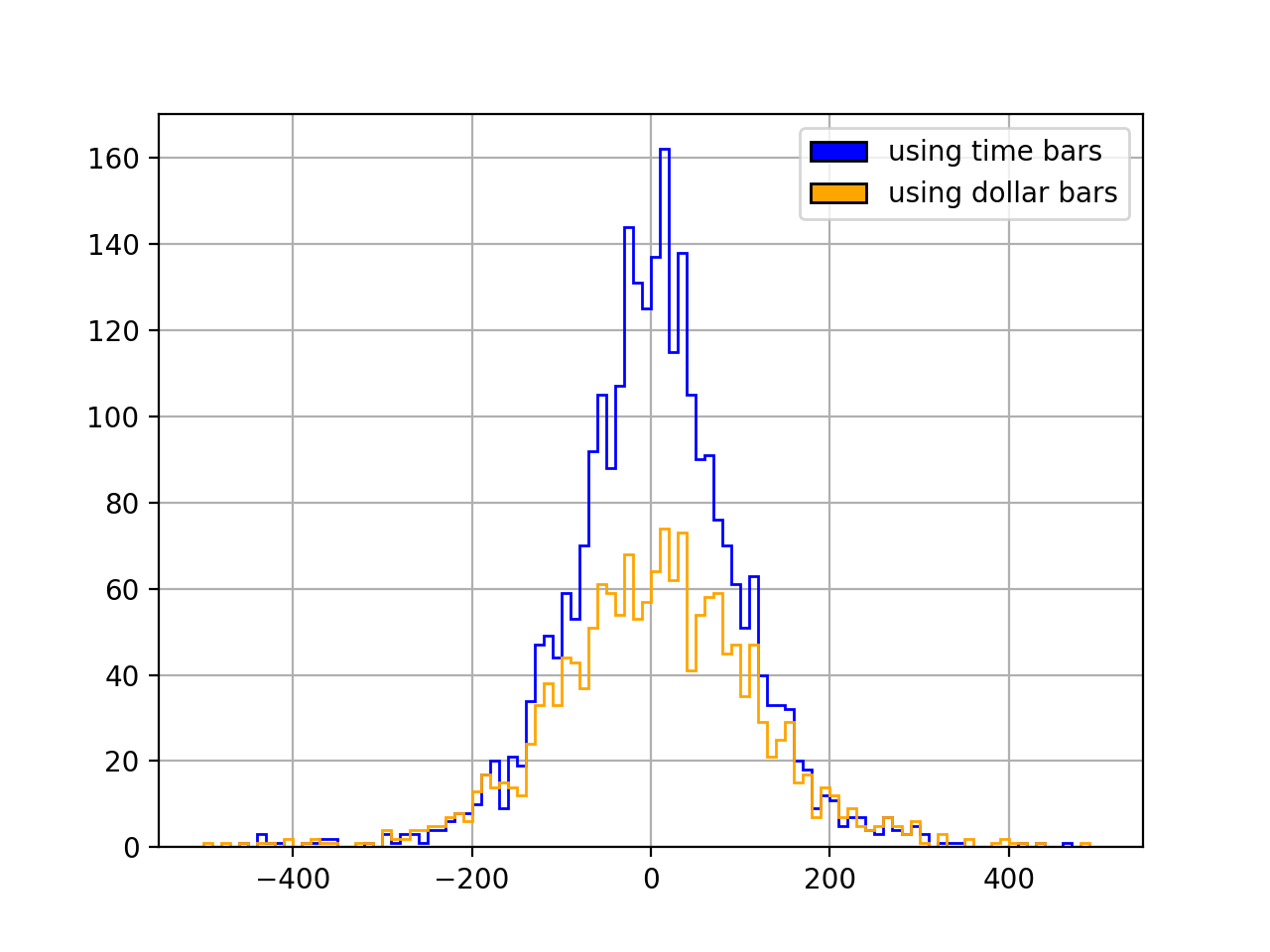
Have we made BOVA11 returns more normal by using dollar bars? Here is the code to check that:
## check if dollar bars improved normality
# testing and plotting parameters
alpha=1e-3rnge=(-500,500)bins=100# time bars
y1=df['PREULT'].diff().dropna().valuesk2,p=normaltest(y1)print('p:',p)ifp<alpha:print('null rejected')else:print('null not rejected')df['PREULT'].diff().hist(bins=bins,range=rnge,histtype='step',color='blue')# dollar bars
y2=bars['closing_price'].diff().dropna().valuesk2,p=normaltest(y2)print('p:',p)ifp<alpha:print('null rejected')else:print('null not rejected')bars['closing_price'].diff().hist(bins=bins,range=rnge,histtype='step',color='orange')# add legend
handles=[Rectangle((0,0),1,1,color=c,ec="k")forcin['blue','orange']]labels=['using time bars','using dollar bars']plt.legend(handles,labels)plt.show()
The null hypothesis here is that the distribution is normal. It is rejected in both cases: neither time bars (p=1.3e-250) nor dollar bars (p=1.5e-125) produce normal returns. But with dollar bars we do get a more normal-looking, less “spiky” distribution:
## check if dollar bars reduced autocorrelation
# set number of lags
lags=10# same as de Prado uses
# time bars
y1=df['PREULT'].valuesac_test=acorr_ljungbox(y1,lags=[lags])print(ac_test)# dollar bars
y2=bars['closing_price'].valuesac_test=acorr_ljungbox(y2,lags=[lags])print(ac_test)
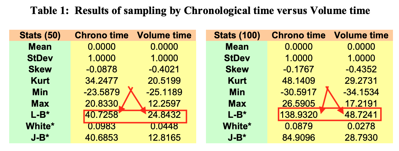
The null hypothesis of zero autocorrelation is rejected in both cases, but the Ljung–Box test statistic is lower with dollar bars (16226) than with time bars (26440). This is similar to what de Prado finds in another of his papers (Flow Toxicity and Liquidity in a High Frequency World, from 2010, on p. 46):
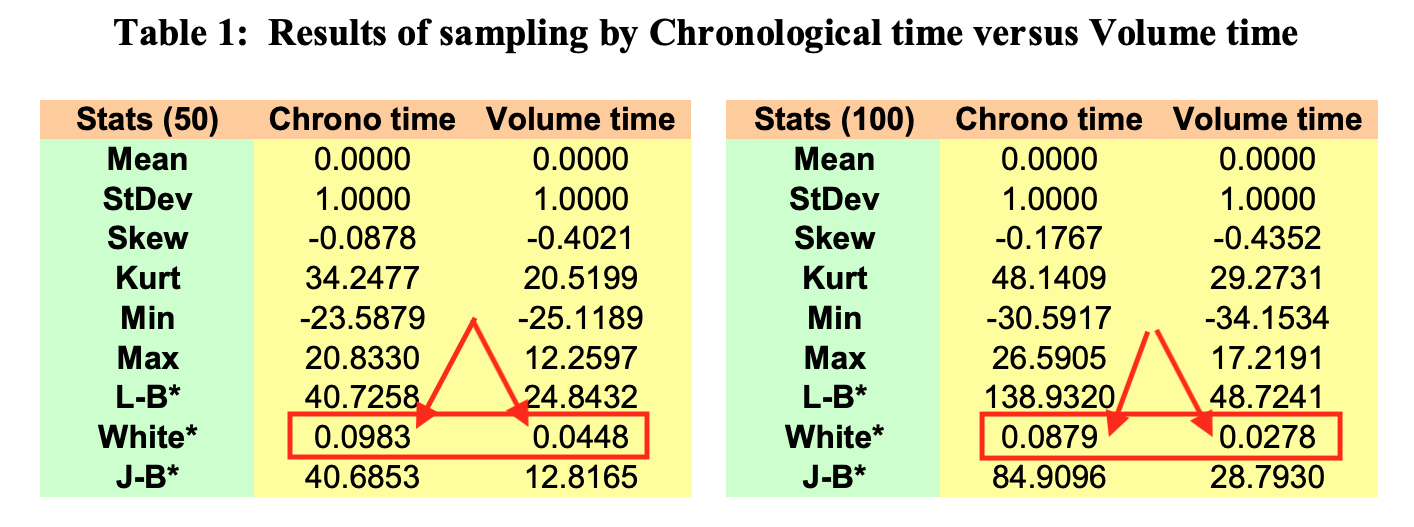
Finally, heteroskedasticity. de Prado (in the same 2010 paper I just mentioned) uses White’s heteroskedasticity test, where you regress your squared residuals against the cross-products of all your features. In the absence of heteroskedasticity the resulting R2 multiplied by the sample size (n) follows a chi-square distribution (with degrees of freedom equal to the number of regressors.)
Now, de Prado has no residuals. He is just building a vector of data to be used in some model later on, same as we are here. So how the heck did he run White’s test? Well, he simply substituted the returns themselves for the residuals. He squared the (standardized) returns and regressed them “against all cross-products of the first 10-lagged series” (p. 46).
I have no idea what the implications of that workaround are. For instance, what if I don’t use an autoregressive model in the end? Maybe with exogenous features I would have no heteroskedasticity to begin with, or maybe I would have heteroskedasticity but the dollar bars wouldn’t help. Heteroskedasticity is a function of the model we are using; as Gujarati notes:
Another source of heteroscedasticity arises from violating Assumption 9 of the classical linear regression model (CLRM), namely, that the regression model is correctly specified. […] very often what looks like heteroscedasticity may be due to the fact that some important variables are omitted from the model. Thus, in the demand function for a commodity, if we do not include the prices of commodities complementary to or competing with the commodity in question (the omitted variable bias), the residuals obtained from the regression may give the distinct impression that the error variance may not be constant. But if the omitted variables are included in the model, that impression may disappear. (Basic Econometrics, p. 367)
Some Monte Carlos might be useful here. We could generate synthetic price data, get the returns, see what happens to the variance of the residuals under different model specifications, and see how heteroskedasticity affects predictive performance. But that’s more work than I’m willing to put into this blog post. Also, de Prado’s algorithms are in charge of Abu Dhabi’s US$ 828 billion sovereign fund. With that much skin in the game he probably knows what he is doing. (On top of that, he has an Erdős 2 and an Einstein 4.) So here I choose to just trust de Prado. Sorry again, reviewer 2.
Here’s the code:
## check if dollar bars reduced heteroskedasticity
# (statsmodels' het_white method returns an
# assertion error, so I had to do it "manually")
defcheck_het(df,price_col):lags=10# same as de Prado used
# get returns
df['DIFF']=df[price_col].diff()# standardize returns
scaler=StandardScaler()df['DIFF']=scaler.fit_transform(df['DIFF'].values.reshape(-1,1))# square standardized returns
df['DIFF']=df['DIFF'].map(lambdax:x**2)# make lags
forlaginrange(1,lags+1):df['LAG_'+str(lag)]=df['DIFF'].shift(lag)df=df.dropna()y1=df['DIFF'].valuesx1=df[[eforeindf.columnsif'LAG'ine]].values# make cross-products
poly=PolynomialFeatures(2,include_bias=False)x1=poly.fit_transform(x1)# regress
reg=LinearRegression()reg.fit(x1,y1)R2=reg.score(x1,y1)returnx1.shape[0]*R2,x1.shape[1]# time bars
test_stat,n=check_het(df,'PREULT')print(test_stat,'w/',n,'degrees of freedom')# dollar bars
test_stat,n=check_het(bars,'closing_price')print(test_stat,'w/',n,'degrees of freedom')
In both cases we reject the null hypothesis of homoskedasticity, but the test statistic is lower with dollar bars (1412) than with time bars (2351). (The degrees of freedom are the same in both cases.) Once more we have a result that is similar to what de Prado found (same 2010 paper as before, same table):
(Just for clarity, what de Prado is reporting in this table is the R2 of White’s regression, not White’s test statistic. But the test statistic is just the R2 multiplied by the sample size, which in de Prado’s case is the same for both the time bar series and the dollar bar series. I report the test statistic in my own results because, unlike him, I have different sample sizes.)
was it all worth it?
That’s a hard question to answer because I’m not training any models here. All I have to go by so far are the statistical properties of the BOVA11 returns, which appear to have improved. But does that mean an improvement in predictive performance? I won’t know until I get to the modeling part. So my answer is “stay tuned!”
Brazilian banks commonly use linear regression to appraise real estate: they regress price on features like area, location, etc, and use the resulting model to estimate the market value of the target property. But Brazilian banks do not test the predictive performance of those models, which for all we know are no better than random guesses. That introduces huge inefficiencies in the real estate market. Here we propose a machine learning approach to the problem. We use real estate data scraped from 15 thousand online listings and use it to fit a boosted trees model. The resulting model has a median absolute error of 8,16%. We provide all data and source code.